Structural Econometrics - Assignment 2 Tutorial

Author: Jaepil Lee

Date: 10/23/2022

Model

Data

Estimation

We aim to replicate a table below by using monthly data from 1960-1 to 2020-12.

Note: The panels of Table III that this assignment asks you to replicate appear in their errata published in 1984.

ENV["COLUMNS"]=100; ENV["LINES"]=1000
# Importing packages...
using Pkg; Pkg.activate("./..");
using Distributions, Statistics, Random, HypothesisTests,
      LinearAlgebra, Distances, SharedArrays, 
      Optim, ForwardDiff, NLSolversBase, 
      Plots, Printf, LaTeXStrings, PlotThemes,
      CSV, DataFrames, TimeSeries, Dates,
      FredApi, FredData;

  Activating project at `c:\Users\jaepi\OneDrive\Documents\GitHub\Prof_Miller_structural_econometrics`

Definition (Bruce Hansen, p.416)

Let $\beta$ be a $k\times1$ vector, $f_i(\beta)$ be a $l\times1$ moments, and $W$ be a $l\times l$ positive definite weighting matrix. Define the GMM criterion function $J(\beta)$ as $$ J(\beta) = N \left(\frac{1}{N}\sum_{i=1}^N f_i(\beta)\right)' W \left(\frac{1}{N}\sum_{i=1}^N f_i(\beta)\right). $$ The GMM estimator is $$ \hat{\beta}_{gmm} = \underset{\beta}{\arg\min}\; J(\beta). $$

Proposition (Bruce Hansen, p.432)

Under general regularity conditions, $\sqrt{N}(\hat{\beta}_{gmm}-\beta_0) \xrightarrow[]{d} N(0,V_\beta)$ where $$ \begin{align*} V_\beta &= (Q'WQ)^{-1}(Q'W\Omega WQ)(Q'WQ)^{-1}\\ \Omega &= \mathbb{E}(f_i f_i') \\ Q &= \mathbb{E}\left[\frac{\partial}{\partial \beta'}f_i(\beta)\right]. \end{align*} $$ If $W$ is efficient, $V_\beta = (Q'\Omega^{-1} Q)^{-1}$.

Note that when you compute standard errors for $\hat{\beta}_{gmm}$, you must divide $V_\beta$ by $N$! $V_\beta$ is the variance for $\sqrt{N}(\hat{\beta}_{gmm}-\beta)$, not $\hat{\beta}_{gmm}$ .

Two-step GMM (Bruce Hansen, p.444)

In order to construct the efficient GMM estimator, we need to know what is the optimal $W$ in our model. In LIV, we know that $W=(Z'Z)^{-1}$. If the optimal weighting matrix $W=\Omega^{-1}$ is unknown, then we can first estimate $W$ with a standard GMM routine (say, by setting $W=I$), and then do the GMM routine again with $W=\hat{\Omega}^{-1}$.

Programming

In this case, we can simply code GMM as follows:

1. Set some weighting matrix $W$. In our example, for the just-identified case, use $W=I$ and for the over-identified case, use $W=(Z'Z)^{-1}$.
2. Construct the GMM criterion function. It is obj_IV in my code.
3. Ask the computer to minimize the criterion function for you. The minimizer is your $\hat{\beta}_{gmm}$.
4. Compute $Q$ and $\Omega$.
   • If you are using a two-step GMM, then repeat step 3 and 4 by setting $W=\hat{\Omega}^{-1}$
5. Compute the asymptotic variance $V_\beta$.
6. Compute standard errors with $\textbf{sqrt}.(\textbf{diag}(\mathbf{V_\beta}/N))$

There is small difference between two-step GMM and One-step GMM with $W=(Z'Z)^{-1}$ because two-step GMM estimated $W$. As you increase $N$, this difference will disappear.

One could also iterate steps as many times as you wish until the updated $\hat{\beta}_{gmm}$ converges. This is called Iterated GMM. Note, however, the two-step GMM is already asymptotically efficient. You might want to use iterated GMM if you think the estimates are suffering from small sample.

Programming

1. Set some weighting matrix $W$. In our example, for the just-identified case, use $W=I$ and for the over-identified case, use $W=(Z'Z)^{-1}$. Also, set some tolerance to declare 'convergence'.
2. Construct the GMM criterion function. It is obj_IV in my code.
3. Ask the computer to minimize the criterion function for you. The minimizer is your $\hat{\beta}_{gmm}$.
4. Compute $Q$ and $\Omega$.
   • Repeat step 3 and 4 by updating $W=\hat{\Omega}^{-1}$ iteratively and until convergence up to some tolerance.
5. Compute the asymptotic variance $V_\beta$.
6. Compute standard errors with $\textbf{sqrt}.(\textbf{diag}(\mathbf{V_\beta}/N))$.

function iterated_GMM(func, γ, y, X, Z; tol=0.001, max_iter=10)

    #=
    func: moment(s)
    X: the matrix of variables that forms moments we wish to make 0
    Z: the matrix orthogonal to moment
    tol: if diff<tol, we claim the update converged
    max_iter: if iter>max_iter, we stop and report what we have so far.
    If max_iter = 2, then it is equivalent to two-step GMM.
    =#

    γ_GMM    = Vector{Vector{Float64}}()
    σ_GMM    = Vector{Vector{Float64}}()
    chi2_vec = Vector{Float64}()
    pval_vec = Vector{Float64}()
    diff_vec = Vector{Float64}()

    N  = size(func(γ, y, X, Z))[1];
    l  = size(func(γ, y, X, Z))[2];
    k  = length(γ);
    df = l-k

    func_vec(γ) = vec(sum(func(γ, y, X, Z),dims=1));

    # First step
    W_1 = I;
    obj_GMM_1(γ) = N * (func_vec(γ)/N)' * W_1 * (func_vec(γ)/N);
    opt_1 = optimize(obj_GMM_1, randn(k), BFGS(), autodiff = :forward);
    γ_GMM_1 = vec(opt_1.minimizer)
    Q_1 = ForwardDiff.jacobian(γ -> func_vec(γ) , γ_GMM_1)/N;
    Ω_1 = func(γ_GMM_1, y, X, Z)'*func(γ_GMM_1, y, X, Z)/N;
    V_GMM_1 = inv(Q_1'*W_1*Q_1)*(Q_1'*W_1*Ω_1*W_1*Q_1)*inv(Q_1'*W_1*Q_1)/N; # remember to divide by N!
    σ_GMM_1 = sqrt.(diag(V_GMM_1))
    chi2 = obj_GMM_1(γ_GMM_1)
    pval = ccdf(Chisq(l-k),obj_GMM_1(γ_GMM_1)) # p-val

    push!(γ_GMM, γ_GMM_1)
    push!(σ_GMM, σ_GMM_1)
    push!(chi2_vec, chi2)
    push!(pval_vec, pval)

    diff = 1e6
    iter = 1
    
    # Iterated GMM
    while (diff > tol) & (iter < max_iter)
        W_opt = inv(Ω_1)
        obj_GMM_2(γ) = N * (func_vec(γ)/N)' * W_opt * (func_vec(γ)/N);
        opt_2 = optimize(obj_GMM_2, randn(k), BFGS(), autodiff = :forward);
        γ_GMM_2 = vec(opt_2.minimizer)
        Q_2 = ForwardDiff.jacobian(γ -> func_vec(γ) , γ_GMM_2)/N;
        Ω_2 = func(γ_GMM_2, y, X, Z)'*func(γ_GMM_2, y, X, Z)/N;
        V_GMM_2 = inv(Q_2'*W_opt*Q_2)*(Q_2'*W_opt*Ω_2*W_opt*Q_2)*inv(Q_2'*W_opt*Q_2)/N; # remember to divide by N!
        σ_GMM_2 = sqrt.(diag(V_GMM_2));
        chi2 = obj_GMM_2(γ_GMM_2)    
        pval = ccdf(Chisq(l-k),obj_GMM_2(γ_GMM_2)) # p-val

        # update
        diff = sqrt(sum((γ_GMM_2-γ_GMM_1).^2))
        Ω_1 = Ω_2
        γ_GMM_1 = γ_GMM_2
        iter += 1

        # record
        push!(diff_vec, diff)
        push!(γ_GMM, γ_GMM_2)
        push!(σ_GMM, σ_GMM_2)
        push!(chi2_vec, chi2)
        push!(pval_vec, pval)
    end

    return γ_GMM, σ_GMM, chi2_vec, df, pval_vec, diff_vec
    
end;

Model review

We consider the following model $$ 1=\mathbb{E}_{t}\left[r_{t+1, k} \beta \frac{u^{\prime}\left(c_{t+1}\right)}{u^{\prime}\left(c_{t}\right)}\right] \equiv \mathbb{E}_{t}\left[r_{t+1, k} MRS_{t+1}\right] $$ where:

• $r_{t+1,k}$ is gross real return on asset $k$
• $\beta \frac{u^{\prime}\left(c_{t+1}\right)}{u^{\prime}\left(c_{t}\right)}$ is marginal rate of substitution (MRS).

Subtracting 1 from each side, we have: $$ 0=\mathbb{E}_{t}\left[r_{t+1, k} \beta \frac{u^{\prime}\left(c_{t+1}\right)}{u^{\prime}\left(c_{t}\right)}-1\right] $$ Under the assumption this model is true, we use data $\{(r_{t+1,k},c_{t},c_{t+1})\}_{t=1}^{T}$ and estimate the parameters of interest.

Let's parametrize the utility function as in Hansen and Singleton (1982). $$ u\left(c_{t}\right)=(1+\alpha)^{-1} c_{t}^{1+\alpha} $$ Notice this utility function exhibits constant relative risk aversion (CRRA) if $\alpha<0$. The population moment becomes a specific nonlinear function of data and parameters: $$ \mathbb{E}_t\left[r_{t+1,k}\beta\left(\frac{c_{t+1}}{c_{t}}\right)^{\alpha}-1\right] = 0 $$ where expectation is taken over the information available at $t$. In other words, any deviation from the equality $r_{t+1,k}\beta(\frac{c_{t+1}}{c_{t}})^\alpha-1=0$ is considered as error.

We wish to use information $\mathbf{x_t} \in I_t$ where $I_t$ the information set known by the agent and $\mathbf{x_t}$ a vector of information observed by econometrician at time $t$. If $\mathbf{x_t}$ is orthogonal to the moment, we can use $\mathbf{x_t}$ as an instrument: $$ \mathbb{E}\left[\mathbf{x_t}\varepsilon_t|I_t\right]:=\mathbb{E}\left[\mathbf{x_t}\cdot\left(r_{t+1,k}\beta\left(\frac{c_{t+1}}{c_{t}}\right)^{\alpha}-1\right)\right]=0 $$

Data

We aim to construct the following data in estimation:

• Real consumption on expenditure on nondurables per capita
• Real consumption on nondurables and services per capita
• Value weighted aggregate stock returns
• Equally weighted aggregate stock returns
• S&P composite returns (Hansen and Singleton uses NYSE)

We use the following data:

• FRED Data: https://fred.stlouisfed.org/series/%5BINDEX NAME].
  • Personal Consumption Expenditures: Nondurable Goods (PCEND)
  • Personal Consumption Expenditures: Nondurable Goods (chain-type price index) (DNDGRG3M086SBEA, PPCEND)
  • Personal Consumption Expenditures: Services (PCES)
  • Personal Consumption Expenditures: Services (chain-type price index) (DSERRG3M086SBEA, PPCES)
  • Consumer Price Index for All Urban Consumers: All Items in U.S. City Average (CPIAUCSL)
  • Population (POPTHM)
  • Population Level (CNP16OV)
  • 1-Year Treasury Constant Maturity Rate (GS1)
  • Real Personal Consumption Expenditures per Capita: Goods: Nondurable goods (A796RX0Q048SBEA)
  • Real Personal Consumption Expenditures per Capita: Services (A797RX0Q048SBEA)
• WRDS Data (CRSP)
  • Value-Weighted Return (Incldues Distributions) (vwretd)
  • Value-Weighted Return (Excluding Dividends) (vwretx)
  • Equal-Weighted Return (Includes Distributions) (ewretd)
  • Equal-Weighted Return (Excluding Dividends) (ewretx)
  • Return on S&P Composite Index (sprtrn)
  • Level on S&P Composite Index (spindx)

#%% Fred Data: API available at https://github.com/markushhh/FredApi.jl
path = "C:/Users/jaepi/OneDrive/Documents/GitHub/Prof_Miller_structural_econometrics/2. Hansen and Singleton, 1982 (GMM)"
set_api_key("...."); # you should get your own API key!

# Monthly Data:
series_code = ["PCEND","DNDGRG3M086SBEA","PCES","DSERRG3M086SBEA","CNP16OV","GS1","CPIAUCSL"];
series_name = ["PCEND","PPCEND","PCES","PPCES","POP","RF","CPI"];

# Quarterly Data:
realND_code = "A796RX0Q048SBEA"; realND_name = "pce_real_ndg";
realS_code = "A797RX0Q048SBEA"; realS_name = "pce_real_svc";

init_date = "1959-12-01"; end_date = "2020-12-01";
Fred_df = DataFrame()
Fred_df[!,:timestamp] = DataFrame(get_symbols("PCEND",init_date,end_date))[1]
Fred_df[!,Symbol.(series_name[1])] = DataFrame(get_symbols("PCEND",init_date,end_date))[2]
for (i,j) in enumerate(series_code)
    Fred_df[!,Symbol(series_name[i])] = DataFrame(get_symbols(j,init_date,end_date))[2]
end

wrds = CSV.read(string(path,"/WRDS.csv"),dateformat="mm/dd/yyyy")[13:end,:]; # 1960/01 to 2020/12

Fred_xt  = TimeArray(Fred_df,timestamp=:timestamp);
wrds_xt  = TimeArray(wrds,timestamp=:DATE);

local API key is set.

Representative Consumer Model: Interpreting estimates from aggregate data

To interpret these results, lifetime utility is: $$ \sum_{t=1}^{\infty} \beta^{t} u\left(c_{t}\right)=(1+\alpha)^{-1} \sum_{t=1}^{\infty} \beta^{t} c_{t}^{1+\alpha} $$

• NDS (nondurables plus services)
• ND (nondurables)
• EWR (NYSE equally weighted average returns)
• VWR (NYSE value weighted average returns)
  • Chemicals, transportation and equipment, and other retail, comprised the three industries.
• Note that:
  • 10 out of 12 specifications in Table III are rejected at the 0.05 level.
  • Since $\alpha>0$ implies convex increasing $u\left(c_{t}\right),$ the 2 remaining specifications in Table III not rejected in a statistical sense do not make economic sense.

Question 1. From 1960 to present, plot the aggregate monthly series of:

• Real consumption on expenditure on nondurables per capita $c_{t}$ and its ratio $c_{t+1} / c_{t}$
• Real consumption on nondurables and services per capita $c_{t}^{*}$ and its ratio $c_{t+1}^{*} / c_{t}^{*}$
• Value weighted aggregate stock returns $r_{t+1}$
• Equally weighted aggregate stock returns $r_{t+1}^{*}$

Real Personal Consumption Expenditure on Nondurables $$ c_t = \frac{\text{Nondurables Consumption}_t * 1\text{e}9}{\text{Nondurables CPI}_t/100}*\frac{1}{\text{Population}_t * 1\text{e}3} $$ Real Personal Consumption Expenditure on Nondurables and Services $$ c_t^* = \left(\frac{\text{Nondurables Consumption}_t * 1\text{e}9}{\text{Nondurables CPI}_t/100}+\frac{\text{Services Consumption}_t * 1\text{e}9}{\text{Services CPI}_t/100}\right)*\frac{1}{\text{Population}_t * 1\text{e}3} $$ Real Value-weighted Return (VWRETD) $$ r_t = \text{Real Value-weighted Return}_t = \frac{1+\text{Value-weighted Return}_t}{\text{CPI}_{t}/\text{CPI}_{t-1}} $$ Real Equal-weighted Return (EWRETD) $$ r_t^* = \text{Real Equal-weighted Return}_t = \frac{1+\text{Equal-weighted Return}_t}{\text{CPI}_t/\text{CPI}_{t-1}} $$ Real S&P Return (SPRTRN) $$ r_t^{**} = \text{Real S\&P Return}_t = \frac{1+\text{S\&P Return}_t}{\text{CPI}_t/\text{CPI}_{t-1}} $$

# FROM FED
PCEND  = Fred_xt[:PCEND].*1_000_000_000; # Billions of Dollars, Seasonally Adjusted Annual Rate
PPCEND = Fred_xt[:PPCEND]./100;          # Index 2012=100, Seasonally Adjusted
PCES   = Fred_xt[:PCES].*1_000_000_000;  # Billions of Dollars, Seasonally Adjusted Annual Rate
PPCES  = Fred_xt[:PPCES]./100;           # Index 2012=100, Seasonally Adjusted
POP    = Fred_xt[:POP].*1000;            # Thousands of Persons
RF     =(Fred_xt[:RF]./100)[2:end];      # Percent, Not Seasonally Adjusted from 1960/01 to 2020/12
CPI    = Fred_xt[:CPI]./100;             # CPI

# FROM WRDS
VWRETD = wrds[:vwretd];                  # Value-Weighted Return (Incldues Distributions)  (vwretd)
VWRETX = wrds[:vwretx];                  # Value-Weighted Return (Excluding Dividends)     (vwretx)
EWRETD = wrds[:ewretd];                  # Equal-Weighted Return (Includes Distributions)  (ewretd)
EWRETX = wrds[:ewretx];                  # Equal-Weighted Return (Excluding Dividends)     (ewretx)
SPRTRN = wrds[:sprtrn];                  # Return on S&P Composite Index (sprtrn)
SPINDX = wrds[:spindx];                  # Level on S&P Composite Index (spindx)

# Real Personal Consumption Expenditure
rPCENDpc = PCEND./(PPCEND.*POP);
rPCESpc = PCES./(PPCES.*POP);
rPCEpc = rPCENDpc .+ rPCESpc;
rPCENDpcRatio = rPCENDpc./lag(rPCENDpc,1,padding=false);
rPCEpcRatio = rPCEpc./lag(rPCEpc,1,padding=false);
TimeSeries.rename!(rPCENDpc, :rPCENDpc);
TimeSeries.rename!(rPCESpc, :rPCESpc);
TimeSeries.rename!(rPCEpc, :rPCEpc);
TimeSeries.rename!(rPCENDpcRatio, :rPCENDpcRatio);
TimeSeries.rename!(rPCEpcRatio, :rPCEpcRatio);

# Inflation and Risk-free Return
INF = CPI./lag(CPI,1,padding=false);
nRF = RF; # Nominal risk-free rate
TimeSeries.rename!(INF, :INF);
TimeSeries.rename!(nRF, :nRF);

# S&P market return
rVWRETD = (1 .+ VWRETD) ./ INF
rEWRETD = (1 .+ EWRETD) ./ INF
rSPRTRN = (1 .+ SPRTRN) ./ INF
TimeSeries.rename!(rVWRETD, :rVWRETD);
TimeSeries.rename!(rEWRETD, :rEWRETD);
TimeSeries.rename!(rSPRTRN, :rSPRTRN);

gr(fmt=png);
min_date = Dates.Date(1960,1,1)
max_date = Dates.Date(2020,12,1)
p1 = plot(rPCENDpc,label="",
          title=L"C_{t}: \textrm{PCEND per capita (Deflated)}",
          xlims = Dates.value.([min_date, max_date]),
          xticks= min_date:Year(10):max_date)
p2 = plot(rPCENDpcRatio,label="",
          title=L"C_{t+1}/C_{t}: \textrm{PCEND per capita Ratio}",
          xlims = Dates.value.([min_date, max_date]),
          xticks= min_date:Year(10):max_date)
p3 = plot(rPCEpc,label="",
          title=L"C_{t}^{*}: \textrm{PCE per capita (Deflated)}",
          xlims = Dates.value.([min_date, max_date]),
          xticks= min_date:Year(10):max_date)
p4 = plot(rPCEpcRatio,label="",
          title=L"C_{t+1}^{*}/C_{t}^{*}: \textrm{PCE per capita Ratio}",
          xlims = Dates.value.([min_date, max_date]),
          xticks= min_date:Year(10):max_date)
fig_c=plot(p1, p2, p3, p4, layout = @layout([p1 p3; p2 p4]), label=["" ""],size=(1200,800))

p1 = plot(rVWRETD,label="",
          title=L"r_{t} \textrm{: Value-weighted Return}",
          xlims = Dates.value.([min_date, max_date]),
          xticks= min_date:Year(15):max_date)
p2 = plot(rEWRETD,label="",
          title=L"r_{t}^{*} \textrm{: Equal-weighted Return}",
          xlims = Dates.value.([min_date, max_date]),
          xticks= min_date:Year(15):max_date)
p3 = plot(rSPRTRN,label="",
          title=L"r_{t}^{**} \textrm{: S\&P Return}",
          xlims = Dates.value.([min_date, max_date]),
          xticks= min_date:Year(15):max_date)
fig_r=plot(p1, p2, p3, layout = @layout([p1 p2 p3]), label=["" ""],size=(1200,360))

Question 2. Replicate the two panels of Table III from Hansen and Singleton (1984) to the extent you can with their subsample (1960-1 to 1978.12) and the instruments they used.

Before we get into Table III, let's see how we would replicate Table I:

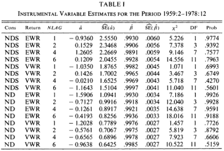
Let's consider the first line. We are using NDS, EWR, in the moment function and one their lagged terms as instruments. $$ \mathbb{E}\left[\begin{pmatrix} 1\\ \frac{c_t^{*}}{c_{t-1}^{*}}\\ r_{t}^{*} \end{pmatrix} \cdot \left(r_{t+1}^{*}\beta\left(\frac{c_{t+1}^{*}}{c_t^{*}}\right)^{\alpha}-1\right)\right] = 0 \\ $$

# TABLE 1: EXAMPLE
# CONSUMPTION: NDS
# RETURN:      EWR
# NLAG:        1

C⃰ = values(rPCEpcRatio)[2:end];
r⃰ = values(rEWRETD)[2:end];
X = [C⃰ r⃰]; # N×2 matrix

C⃰_L1 = values(lag(rPCEpcRatio,1,padding=false))[1:end];
r⃰_L1 = values(lag(rEWRETD,1,padding=false))[1:end];
Z = [ones(length(C⃰_L1)) C⃰_L1 r⃰_L1]; # N×l matrix

function f_HS_TABLE1_EXAMPLE(γ, y, X, Z)
    #= 
    γ: parameters. γ[1]=α, γ[2]=β
    X: the matrix of variables that forms moments we wish to make 0
    Z: the matrix orthogonal to moment
    We want to have a N×3 vector
    =#
    C⃰, r⃰ = X[:,1], X[:,2]
    return (r⃰ .* γ[2] .* C⃰.^γ[1] .- y) .* Z # (N×1) ⊗ (N×3)
end;
γ_GMM, σ_GMM, chi2_vec, df, pval_vec, diff_vec = iterated_GMM(f_HS_TABLE1_EXAMPLE, rand(2), ones(length(C⃰)), X, Z; tol=1e-8, max_iter=100);

Note that the code returns p-values as pval_vec, not "Prob". In Hansen and Singleton (1982), they reported (1-p-value) in the Prob column.

print("Hansen-Singleton GMM Replication: Table I \n")
print("Instrument Variable Estimates for the Period 1960:1 to 2020:12 \n")
print("One-step GMM \n")
print("Consumption | Return | NLAG |    α    |   se(α)   |    β    |   se(α)   |   χ²   | DF | p-value ||\n")
@printf("NDS         | EWR    | 1    | %7.4f | (%7.5f) | %7.4f | (%7.5f) | %6.4f | %2i | %6.4f  ||\n", 
        γ_GMM[1][1], σ_GMM[1][1],γ_GMM[1][2], σ_GMM[1][2], chi2_vec[1], df, pval_vec[1])

Hansen-Singleton GMM Replication: Table I 
Instrument Variable Estimates for the Period 1960:1 to 2020:12 
One-step GMM 
Consumption | Return | NLAG |    α    |   se(α)   |    β    |   se(α)   |   χ²   | DF | p-value ||
NDS         | EWR    | 1    | -6.8895 | (4.25675) |  0.9991 | (0.00618) | 0.0000 |  1 | 0.9986  ||

print("Hansen-Singleton GMM Replication: Table I \n")
print("Instrument Variable Estimates for the Period 1960:1 to 2020:12 \n")
print("Two-step GMM \n")
print("Consumption | Return | NLAG |    α    |   se(α)   |    β    |   se(α)   |   χ²   | DF |  p-value ||\n")
@printf("NDS         | EWR    | 1    | %7.4f | (%7.5f) | %7.4f | (%7.5f) | %6.4f | %2i |  %6.4f  ||\n", 
        γ_GMM[2][1], σ_GMM[2][1], γ_GMM[2][2], σ_GMM[2][2], chi2_vec[2], df, pval_vec[2])

Hansen-Singleton GMM Replication: Table I 
Instrument Variable Estimates for the Period 1960:1 to 2020:12 
Two-step GMM 
Consumption | Return | NLAG |    α    |   se(α)   |    β    |   se(α)   |   χ²   | DF |  p-value ||
NDS         | EWR    | 1    | -7.9837 | (4.40576) |  1.0013 | (0.00603) | 1.1553 |  1 |  0.2824  ||

print("Hansen-Singleton GMM Replication: Table I \n")
print("Instrument Variable Estimates for the Period 1960:1 to 2020:12 \n")
print("Iterated GMM until convergence with tolerance 1e-8 \n")
print("Consumption | Return | NLAG |    α    |   se(α)   |    β    |   se(α)   |   χ²   | DF |  p-value | Iteration ||\n")
@printf("NDS         | EWR    | 1    | %7.4f | (%7.5f) | %7.4f | (%7.5f) | %6.4f | %2i |  %6.4f  | %5i     ||\n", 
        γ_GMM[end][1], σ_GMM[end][1], γ_GMM[end][2], σ_GMM[end][2], chi2_vec[end], df, pval_vec[end], size(γ_GMM)[1])

Hansen-Singleton GMM Replication: Table I 
Instrument Variable Estimates for the Period 1960:1 to 2020:12 
Iterated GMM until convergence with tolerance 1e-8 
Consumption | Return | NLAG |    α    |   se(α)   |    β    |   se(α)   |   χ²   | DF |  p-value | Iteration ||
NDS         | EWR    | 1    | -8.3454 | (4.50449) |  1.0017 | (0.00613) | 0.7906 |  1 |  0.3739  |    16     ||

Let's replicate Table III (Finally!)

Panel A

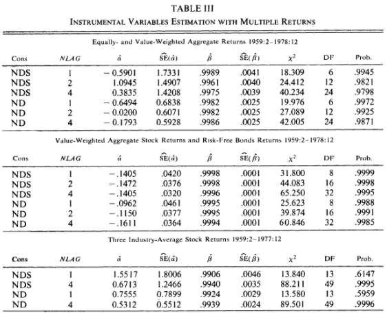
There is one more complication here: we now have two sets of orthogonality conditions. The first line estimates of Table III uses equally- and value-weighted returns, with one lag for each of the consumption ration and equally- and value-weighted returns. This is a set of 8 population moment conditions in 2 parameters ($\alpha,\beta$).

$$ \begin{align*} \mathbb{E}\left[\begin{pmatrix} 1\\ \frac{c_t}{c_{t-1}}\\ r_{t}^*\\ r_{t} \end{pmatrix} \cdot \left(r_{t+1}^*\beta\left(\frac{c_{t+1}^*}{c_t^*}\right)^{\alpha}-1\right)\right] &= 0 \\ \mathbb{E}\left[\begin{pmatrix} 1\\ \frac{c_t}{c_{t-1}}\\ r_{t}^*\\ r_{t} \end{pmatrix} \cdot \left(r_{t+1}\beta\left(\frac{c_{t+1}^*}{c_t^*}\right)^{\alpha}-1\right)\right] &= 0 \end{align*} $$

The degree of freedom (DF) is 2*(1+(NLAG of consumption ratio)+(NLAG of EWR)+(NLAG of VWR))-2

• NLAG=1: $2\times(1+1+1+1)-2=6$
• NLAG=2: $2\times(1+2+2+2)-2=12$
• NLAG=4: $2\times(1+4+4+4)-2=24$

# TABLE 3: EXAMPLE
# CONSUMPTION: NDS
# RETURN: EWR & VWR
# NLAG: 1

C⃰ = values(rPCEpcRatio)[2:end];
r  = values(rVWRETD)[2:end];
r⃰ = values(rEWRETD)[2:end];
X = [C⃰ r r⃰];

C⃰_L1 = values(lag(rPCEpcRatio,1,padding=false));
r_L1  = values(lag(rVWRETD,1,padding=false));
r⃰_L1 = values(lag(rEWRETD,1,padding=false));
Z = [ones(length(C⃰_L1)) C⃰_L1 r_L1 r⃰_L1];

function f_HS_TABLE3_EXAMPLE(γ, y, X, Z)
    #= 
    γ: parameters. γ[1]=α, γ[2]=β
    X: the matrix of variables that forms moments we wish to make 0
    Z: the matrix orthogonal to moment
    We want to have a N×8 vector
    =#
    C⃰, r, r⃰ = X[:,1], X[:,2], X[:,3];
    m1 = (r⃰ .* γ[2] .* C⃰.^γ[1] - y) .* Z # (N×1) ⊗ (N×4)
    m2 = (r  .* γ[2] .* C⃰.^γ[1] - y) .* Z # (N×1) ⊗ (N×4)
    return [m1 m2]
end;

Panel B

In Hansen and Singleton (1984), they describe how they used the nominal risk-free returns:

$$ \begin{align*} \mathbb{E}\left[\begin{pmatrix} 1\\ \frac{c_t}{c_{t-1}}\\ r_{t}\\ \frac{R_{t+1}^f}{R_{t}^f}\\ \frac{R_{t}^f}{R_{t-1}^f} \end{pmatrix} \cdot \left(r_{t+1}\beta\left(\frac{c_{t+1}^*}{c_t^*}\right)^{\alpha}-1\right)\right] &= 0 \\ \mathbb{E}\left[\begin{pmatrix} 1\\ \frac{c_t}{c_{t-1}}\\ r_t \\ \frac{R_{t+1}^f}{R_{t}^f}\\ \frac{R_{t}^f}{R_{t-1}^f} \end{pmatrix} \cdot \left(R_{t+1}^f \beta\left(\frac{c_{t+1}}{c_t}\right)^{\alpha}-1\right)\right] &= 0 \end{align*} $$

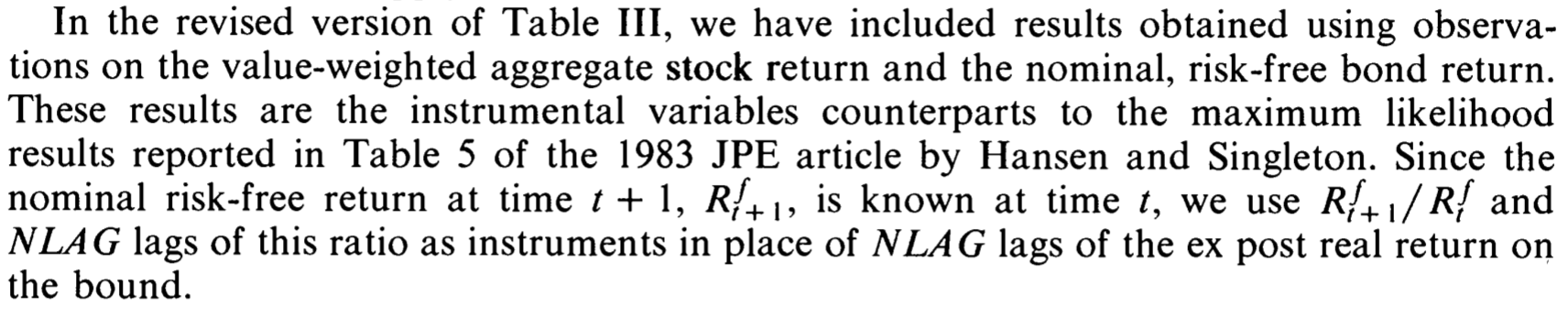
Their claim is that the degree of freedom is 2* [constant + (risk-free ratio + NLAG for risk-free ratio) + (NLAG for consumption ratio) + (NLAG for VWR)]-2

• NLAG=1: $2\times(1+(1+1)+1+1)-2=8$
• NLAG=2: $2\times(1+(1+2)+2+2)-2=14$
• NLAG=4: $2\times(1+(1+4)+4+4)-2=26$

(Credit to Christine Dabbs) However, it seems like Hansen and Singleton double-counted the number of risk-free ratios. They have df = 8, 16, 32. These numbers are replicable if we counted degree of freedoms as:

2* [constant + 2*(NLAG for risk-free ratio) + (NLAG for consumption ratio) + (NLAG for VWR)]-2

• NLAG=1: $2\times(1+2*1+1+1)-2=8$
• NLAG=2: $2\times(1+2*2+2+2)-2=16$
• NLAG=4: $2\times(1+2*4+4+4)-2=32$

Question 3

Here, you are now estimating 4 parameters, $(\alpha_1,\beta_1,\alpha_2,\beta_2)$. You may want to find $(\alpha_1,\beta_1)$ only with data from 1960.1 to 1978.12 and $(\alpha_2,\beta_2)$ with data from 1979.1 and onward. You can change f_HS_TABLE3_EXAMPLE to do this exercise. You can only use data from 1960.1 to 1978.12 for m1 and use data from 1979.1 to 2020.12 for m2. You may also want to use $4\times1$ vector $\vec{\gamma}$. This is your 'unconstrained' GMM.

Now, you are asked to test $(\alpha_1,\beta_1)=(\alpha_2,\beta_2)$. The following theorem will be helpful:

Theorem (Professor Miller's Lecture Notes, slide 17)

Let $J_{un}$ be the unconstrained GMM criterion function with $l_1$ orthogonality conditions and $k_1$ parameters. Let $J_{con}$ be the constrained GMM criterion function with $l_2$ orthogonality conditions and $k_2$ parameters. Then, $$ J_{con} - J_{un} \overset{d}{\longrightarrow} \chi^2_{(l_2-k_2)-(l_1-k_1)}. $$

Additionally, you might be able to test models with more parameters in more time frames, say, before/after the financial crisis in 2008 and before/after COVID-19. To do so, you may need more instruments using more lagged variables.

Question 4 and 5

I will leave questions 4 and 5 for you to explore. Now you have basic codes to run, I am sure you can easily modify code and get the estimates.

Question 6

Let’s come back to data and think about big picture here. Hansen and Singleton (1982) assumes that we have a stationary environment. Test whether any of these series we considered in question 1 have a unit root. (You should read about unit root tests first.) Is there evidencethat these series are not stationary and ergodic?

I use Augmented Dickey-Fuller (ADF) Test. I will let you discuss whether you think time series data we used are stationary and ergodic.

(Not graded) TA's conjecture: Try ADF tests with i) a constant, ii) a trend, iii) a trend and trend squared. What do these tests tell you? If Hansen and Singleton (1982) requires stationarity, how would you incorporate the findings to your model?

varDF = DataFrame(varname=Vector{String}(),
                varsymbol=Vector{Symbol}(),
                vardata=Vector{TimeArray}())
varDF=vcat(varDF,DataFrame(varname="PCE per Capita (deflated)",varsymbol=:rPCEpc,vardata=rPCEpc))
varDF=vcat(varDF,DataFrame(varname="PCEND per Capita (deflated)",varsymbol=:rPCENDpc,vardata=rPCENDpc))
varDF=vcat(varDF,DataFrame(varname="PCE per Capita (deflated) ratio",varsymbol=:rPCEpcRatio,vardata=rPCEpcRatio))
varDF=vcat(varDF,DataFrame(varname="PCEND per Capita (deflated) ratio",varsymbol=:rPCENDpcRatio,vardata=rPCENDpcRatio))
varDF=vcat(varDF,DataFrame(varname="Real Equal-weighted Returns",varsymbol=:rEWRETD,vardata=rEWRETD))
varDF=vcat(varDF,DataFrame(varname="Real Value-Weighted Returns",varsymbol=:rVWRETD,vardata=rVWRETD))
varDF=vcat(varDF,DataFrame(varname="Real S&P Returns",varsymbol=:rSPRTRN,vardata=rSPRTRN))
for i in 1:4
    name = varDF[:varname][i]
    symbol = varDF[:varsymbol][i]
    data = varDF[:vardata][i]
    data = DataFrame(data)[!,symbol][2:end]
    print("ADF Test: $name \n")
    print("        | Coefficient |  Statistic  | p-value | \n")
    for lags = [1,2,4,6]
        stat = ADFTest(data, :none, lags).stat
        coef = ADFTest(data, :none, lags).coef
        pval = pvalue(ADFTest(data, :none, lags))
        print("NLAGS:$lags |")
        @printf(" %11.8f | %11.8f |  %6.4f | \n", coef, stat, pval)
    end
    print("\n")
end

ADF Test: PCE per Capita (deflated) 
        | Coefficient |  Statistic  | p-value | 
NLAGS:1 |  0.00085897 |  2.85174757 |  0.9996 | 
NLAGS:2 |  0.00114181 |  3.93944023 |  1.0000 | 
NLAGS:4 |  0.00131477 |  4.43821690 |  1.0000 | 
NLAGS:6 |  0.00155524 |  5.11989688 |  1.0000 | 

ADF Test: PCEND per Capita (deflated) 
        | Coefficient |  Statistic  | p-value | 
NLAGS:1 |  0.00128219 |  3.41828302 |  1.0000 | 
NLAGS:2 |  0.00164927 |  4.51403679 |  1.0000 | 
NLAGS:4 |  0.00176250 |  4.68681891 |  1.0000 | 
NLAGS:6 |  0.00189009 |  4.85354412 |  1.0000 | 

ADF Test: PCE per Capita (deflated) ratio 
        | Coefficient |  Statistic  | p-value | 
NLAGS:1 | -0.00004487 | -0.13793068 |  0.6365 | 
NLAGS:2 | -0.00004233 | -0.14274545 |  0.6348 | 
NLAGS:4 | -0.00001400 | -0.05039685 |  0.6673 | 
NLAGS:6 |  0.00003243 |  0.12242773 |  0.7235 | 

ADF Test: PCEND per Capita (deflated) ratio 
        | Coefficient |  Statistic  | p-value | 
NLAGS:1 | -0.00008071 | -0.17065202 |  0.6247 | 
NLAGS:2 | -0.00008845 | -0.21832532 |  0.6071 | 
NLAGS:4 | -0.00002615 | -0.07215051 |  0.6598 | 
NLAGS:6 |  0.00001318 |  0.03774306 |  0.6967 | 

for i in 5:size(varDF)[1]
    name = varDF[:varname][i]
    symbol = varDF[:varsymbol][i]
    data = varDF[:vardata][i]
    data = DataFrame(data)[!,symbol][2:end]
    print("ADF Test: $name \n")
    print("        | Coefficient |  Statistic  | p-value | \n")
    for lags = [1,2,4,6]
        stat = ADFTest(data, :none, lags).stat
        coef = ADFTest(data, :none, lags).coef
        pval = pvalue(ADFTest(data, :none, lags))
        print("NLAGS:$lags |")
        @printf(" %11.8f | %11.8f |  %6.4f | \n", coef, stat, pval)
    end
    print("\n")
end

ADF Test: Real Equal-weighted Returns 
        | Coefficient |  Statistic  | p-value | 
NLAGS:1 | -0.00132420 | -0.55045316 |  0.4753 | 
NLAGS:2 | -0.00079946 | -0.34919278 |  0.5569 | 
NLAGS:4 | -0.00043876 | -0.20011743 |  0.6139 | 
NLAGS:6 | -0.00026769 | -0.12388804 |  0.6416 | 

ADF Test: Real Value-Weighted Returns 
        | Coefficient |  Statistic  | p-value | 
NLAGS:1 | -0.00087740 | -0.43674454 |  0.5219 | 
NLAGS:2 | -0.00047429 | -0.25249830 |  0.5942 | 
NLAGS:4 | -0.00025356 | -0.14288880 |  0.6348 | 
NLAGS:6 | -0.00013940 | -0.07966280 |  0.6572 | 

ADF Test: Real S&P Returns 
        | Coefficient |  Statistic  | p-value | 
NLAGS:1 | -0.00082647 | -0.42204541 |  0.5279 | 
NLAGS:2 | -0.00043780 | -0.24036229 |  0.5988 | 
NLAGS:4 | -0.00022709 | -0.13279936 |  0.6384 | 
NLAGS:6 | -0.00012772 | -0.07558289 |  0.6586 | 

References:

• Professor Miller's Lecture Note Chapters 3 and 12
• Bruce Hansen's econometrics textbook
• Hansen, Lars Peter, and Kenneth J. Singleton. "Generalized instrumental variables estimation of nonlinear rational expectations models." Econometrica: Journal of the Econometric Society (1982): 1269-1286.
• Hansen, Lars Peter. "Large sample properties of generalized method of moments estimators." Econometrica: Journal of the econometric society (1982): 1029-1054.
• Newey, Whitney K., and Daniel McFadden. "Large sample estimation and hypothesis testing." Handbook of econometrics 4 (1994): 2111-2245.